キンラン、ギンラン、ベイジアン・ネットワーク [科学、数学]
今年も、こども自然公園にキンランとギンランが咲いていました。
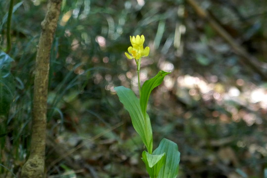
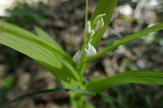
今まで気が付きませんでしたが、追分市民の森にも、キンランとギンランが咲いていました。


キンラン、ギンランとは、関係ないのですがベイジアン・ネットワーク
(キンラン、ギンランも地面の中では菌根菌(きんこんきん、mycorrhizal fungi)のネットワークを作っているらしいです。)
最近ベイジアン・ネットワークの良いテキストを見つけました。
Understanding Bayesian Networks with Examples in R
http://www.bnlearn.com/about/teaching/slides-bnshort.pdf
このスライド中のHands-On ExamplesのCase Studyが、とてもわかりやすいです。
Causal Protein-Signaling Networks Derived from Multiparameter Single-Cell Data (http://science.sciencemag.org/content/308/5721/523)に掲載されているネットワークをRのbnlearnというパッケージを利用して作っていきます。
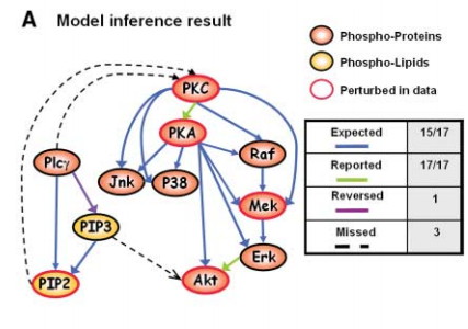
Causal Protein-Signaling Networks Derived from Multiparameter Single-Cell Data: Fig. 3. Bayesian network inference
results. 22 APRIL 2005 VOL 308 SCIENCE www.sciencemag.org
データは、このページからダウンロードできます。
Bayesian Networks with Examples in R
http://www.bnlearn.com/book-crc/
Sachs' raw observational data.
Sachs' discretized observational data.
Sachs' complete pre-processed data.
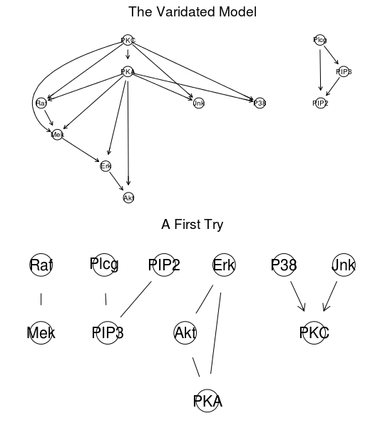
図中の上のようなネットワークにしたいのですが、前処理なしでは、下のようになってしまいます。
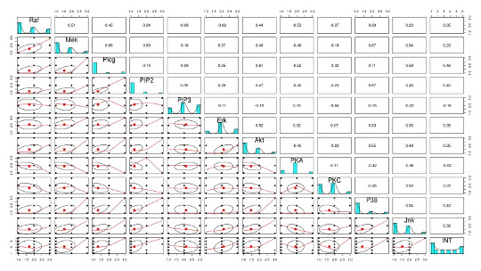
正しいネットワーク作るのには、どのような前処理が必要かを考えるために、元のデータの分布や関連を調べます。
元のデータの分布や関連を見るのは、Rのpsychというパッケージを使うと便利です。
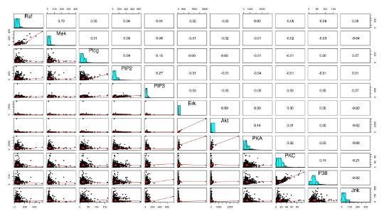
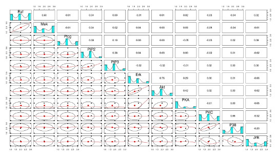
データの分布がかたよっていたり、データ間の関係が線形相関ではないようなので、データを離散化(Discretisation)したりするようです。
bnlearnには、離散化のためのHartemink’s algorithmのような関数も用意されていています。
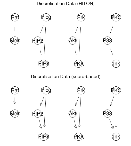
離散化後のデータで、ネットワークを作成
Taking the Interventions into Account
今まで気が付きませんでしたが、追分市民の森にも、キンランとギンランが咲いていました。
キンラン、ギンランとは、関係ないのですがベイジアン・ネットワーク
(キンラン、ギンランも地面の中では菌根菌(きんこんきん、mycorrhizal fungi)のネットワークを作っているらしいです。)
最近ベイジアン・ネットワークの良いテキストを見つけました。
Understanding Bayesian Networks with Examples in R
http://www.bnlearn.com/about/teaching/slides-bnshort.pdf
このスライド中のHands-On ExamplesのCase Studyが、とてもわかりやすいです。
Causal Protein-Signaling Networks Derived from Multiparameter Single-Cell Data (http://science.sciencemag.org/content/308/5721/523)に掲載されているネットワークをRのbnlearnというパッケージを利用して作っていきます。
Causal Protein-Signaling Networks Derived from Multiparameter Single-Cell Data: Fig. 3. Bayesian network inference
results. 22 APRIL 2005 VOL 308 SCIENCE www.sciencemag.org
データは、このページからダウンロードできます。
Bayesian Networks with Examples in R
http://www.bnlearn.com/book-crc/
Sachs' raw observational data.
Sachs' discretized observational data.
Sachs' complete pre-processed data.
図中の上のようなネットワークにしたいのですが、前処理なしでは、下のようになってしまいます。
正しいネットワーク作るのには、どのような前処理が必要かを考えるために、元のデータの分布や関連を調べます。
元のデータの分布や関連を見るのは、Rのpsychというパッケージを使うと便利です。
データの分布がかたよっていたり、データ間の関係が線形相関ではないようなので、データを離散化(Discretisation)したりするようです。
bnlearnには、離散化のためのHartemink’s algorithmのような関数も用意されていています。
離散化後のデータで、ネットワークを作成
Taking the Interventions into Account
+ Rのプログラム Bayesian networks Hands-On Examples
# Bayesian networks
# Hands-On Examples
# Case Study: Human Physiology
#
library(bnlearn)
setwd("~/R/bnlearn/crc")
# Exploring the Data
sachs = read.table("sachs.data.txt", header = TRUE)
head(sachs, n = 5)
# A First Try
dag.hiton = si.hiton.pc(sachs, test = "cor", undirected = FALSE)
directed.arcs(dag.hiton)
#undirected.arcs(dag.hiton)
# Compare with the Validated Model
sachs.modelstring =
paste("[PKC][PKA|PKC][Raf|PKC:PKA][Mek|PKC:PKA:Raf][Erk|Mek:PKA]",
"[Akt|Erk:PKA][P38|PKC:PKA][Jnk|PKC:PKA][Plcg][PIP3|Plcg]",
"[PIP2|Plcg:PIP3]")
dag.sachs = model2network(sachs.modelstring)
unlist(compare(dag.sachs, dag.hiton))
par(mfrow=c(2,1))
graphviz.plot(dag.sachs)
graphviz.plot(dag.hiton)
# scatterplots, distributions and correlation
library(psych)
pairs.panels(sachs)
# Discretising Data
# Hartemink’s Information-Preserving Discretisation
dsachs = discretize(sachs, method = "hartemink",
breaks = 3, ibreaks = 60, idisc = "quantile")
head(dsachs)
pairs.panels(dsachs)
# However, HITON is still not working...
dag.hiton = si.hiton.pc(dsachs, test = "x2", undirected = FALSE)
unlist(compare(dag.hiton, dag.sachs))
# ... so we switch to a score-based algorithm ...
dag.hc = hc(dsachs, score = "bde", iss = 10, undirected = FALSE)
unlist(compare(dag.hc, dag.sachs))
graphviz.plot(dag.hc)
# ... and frequentist model averaging to remove spurious arcs.
boot = boot.strength(dsachs, R = 500, algorithm = "hc",
algorithm.args = list(score = "bde", iss = 10))
head(boot[(boot$strength > 0.85) & (boot$direction >= 0.5), ], n = 3)
# Model Averaging from Multiple Searches
nodes = names(dsachs)
# While there is no function in bnlearn that does exactly this, we can
# combine random.graph() and sapply() to generate the random
# starting points and call hc() on each of them.
startlist = random.graph(nodes = nodes, method = "ic-dag",
num = 500, every = 50)
netlist = lapply(startlist,
function(net) {
hc(dsachs, score = "bde", iss = 10, start = net)
}
)
# Compare Both Approaches with the Validated Network
start = custom.strength(netlist, nodes = nodes)
avg.start = averaged.network(start)
avg.boot = averaged.network(boot)
unlist(compare(avg.start, dag.sachs))
#tp fp fn
# 3 14 7
unlist(compare(avg.boot, dag.sachs))
#tp fp fn
# 6 11 4
par(mfrow=c(2,1))
graphviz.plot(avg.start)
graphviz.plot(avg.boot)
# Both networks look nothing like the validated network, and in fact fall in
# the same equivalence class.
all.equal(cpdag(avg.boot), cpdag(avg.start))
# The only piece of information we have not taken into account yet are
# the stimulations and the inhibitions, that is, the interventions on the
# variables.
isachs = read.table("sachs.interventional.txt",
header = TRUE, colClasses = "factor")
# A Naive Approach with Whitelists
wh = matrix(c(rep("INT", 11), names(isachs)[1:11]), ncol = 2)
dag.wh = tabu(isachs, whitelist = wh, score = "bde",
iss = 10, tabu = 50)
unlist(compare(subgraph(dag.wh, names(isachs)[1:11]), dag.sachs))
graphviz.plot(dag.wh, highlight = list(nodes = "INT",
arcs = outgoing.arcs(dag.wh, "INT"), col = "darkgrey", fill = "darkgrey"))
# Mixed Observational and Interventional Data
# A more granular way of doing the same thing is to use the mixed observational
# and interventional data posterior score from Cooper & Yoo, which creates an
# implicit intervention binary node for each variable.
INT = sapply(1:11, function(x) which(isachs$INT == x) )
nodes = names(isachs)[1:11]
names(INT) = nodes
# Then we perform model averaging of the resulting causal DAGs, with better
# results.
netlist = lapply(startlist, function(net) {
tabu(isachs[, 1:11], score = "mbde", exp = INT, iss = 1,
start = net, tabu = 50)
})
intscore = custom.strength(netlist, nodes = nodes, cpdag = FALSE)
dag.mbde = averaged.network(intscore)
unlist(compare(dag.sachs, dag.mbde))
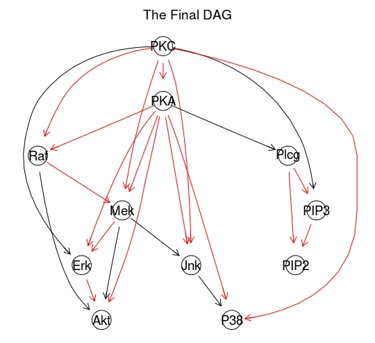
# The Final DAG
graphviz.plot(dag.mbde, highlight = list(arcs = arcs(dag.sachs)))
####
# Using The Protein Network to Plan Experiments
# First, we need to learn the parameters of the BN given the DAG.
isachs = isachs[, 1:11]
for (i in names(isachs))
levels(isachs[, i]) = c("LOW", "AVG", "HIGH")
fitted = bn.fit(dag.sachs, isachs, method = "bayes")
# Then we can proceed to perform queries using gRain, on the original BN
library(gRain)
jtree = compile(as.grain(fitted))
# and on a mutilated BN in which we set Erk to LOW with an ideal
# intervention.
jlow = compile(as.grain(mutilated(fitted, evidence = list(Erk = "LOW"))))
par(mfrow=c(2,1))
plot(jtree)
plot(jlow)
# Interventions and Mutilated Graphs
# Variables That are Downstream are Untouched
querygrain(jtree, nodes = "Akt")$Akt
querygrain(jlow, nodes = "Akt")$Akt
# Causal Inference, Posterior Inference
querygrain(jtree, nodes = "PKA")$PKA
querygrain(jlow, nodes = "PKA")$PKA
jlow = setEvidence(jtree, nodes = "Erk", states= "LOW")
querygrain(jlow, nodes = "PKA")$PKA


コメント 0