因果推論

今週末も横浜は雨だったので、先週に続いて家で、因果推論に親しめるように、Rのtwangとcobaltという、かっこいいパッケージを見つけました。

twang: Toolkit for Weighting and Analysis of Nonequivalent Groups
https://cran.r-project.org/web/packages/twang/index.html

cobalt: Covariate Balance Tables and Plots
https://cran.r-project.org/web/packages/cobalt/index.html

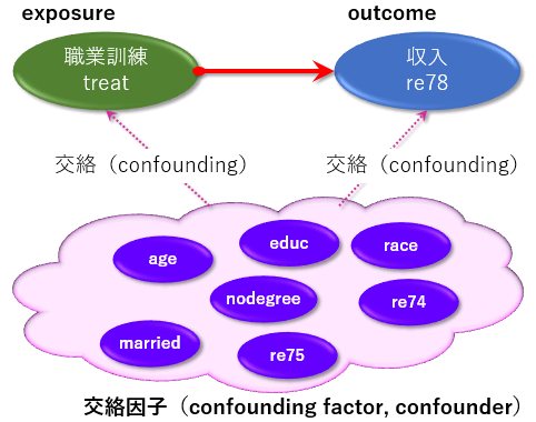
例題として、National Supported Work Demonstration data (米国職業訓練プログラム）のデータから、職業訓練を受けたことと、収入の因果関係を調べます。

職業訓練プログラムのデータには、以下の項目が含まれています。
treat : treatment indicator; 1 if treated in the National Supported Work Demonstration, 0 if from the Current Population Survey (exporsure)
age : age, a numeric vector.
educ : years of education, a numeric vector between 0 and 18.
race : { black | hispaic | white }
married : a binary vector, { 0 | 1 }
nodegree : a binary vector, 1 if no degree, 0 otherwise.
re74 : earnings in 1974, a numeric vector.
re75 : earnings in 1975, a numeric vector.
re78 : earnings in 1978, a numeric vector (outcome variable: 結果変数).

職業訓練を受けたこと ( treat ) が、訓練後（1978年）の年収 ( re78 )に影響をあたえているかどうかを調べたいのですが、収入には職業訓練を受けたかどうかの他にも、年齢や学歴なども影響を与えていることが考えられます。
説明変数（職業訓練をうけたかどうか）と結果変数（1978年の収入）以外の変数で、説明変数や結果変数の両方に相関のあるような変数を交絡因子（confounding factor、confounder）と呼ぶそうです。





---

library(cobalt)

data("lalonde", package = "cobalt")
summary(lalonde)

---

twangパッケージのps関数を使って、傾向スコアモデルを作ります。
全ての人に処置を与えた場合に、どれくらいの底上げ効果があるか、を推定するために、効果の見積方法にATT (Average Treatment effect on Treated )を指定します。
収束条件は、標準化バイアス（Effect Size）の平均と最大を、乱数のシードには、岩波データサイエンスのしきたりに従い1985にしました。

---

library(twang)
set.seed(1985)

covs <- subset(lalonde, select = -c(treat, re78, nodegree, married))

# stopping rule : Effect Size
ps.out <- ps(f.build("treat", covs), data = lalonde,
stop.method = c("es.mean", "es.max"),
estimand = "ATT", n.trees = 1500, verbose = FALSE)

plot(ps.out)

---

plot関数で、収束の状態が確認できます。

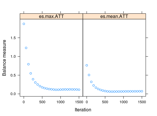
繰り返しを1500回にしましたが、1000回を超えたぐらいで、充分収束しているようです。

---

bal.tab(ps.out, stop.method = "es.mean")

---
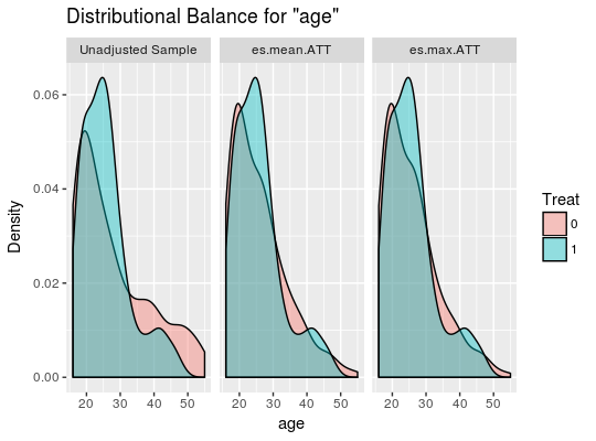
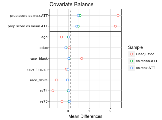
cobaltパッケージのbal.plot　や love.plot を使うと、マッチング前後のバランスをグラフィカルに表示することができます。

---

bal.plot(ps.out, "age", which = "both")

---



---

love.plot(bal.tab(ps.out), threshold = 0.1, which.treat = NULL)

---




ps関数で各オブザベーションの重みが求まるのでそれを元のデータ（lalonde）に付加した後、surveyパッケージを使って、その重みを反映された効果を推定します。

---

library(survey)

lalonde$w <- get.weights(ps.out, stop.method="es.mean")
design.ps <- svydesign(ids=~1, weights=~w, data=lalonde)

res.glm <- svyglm(re78 ~ treat + age + educ + race, design=design.ps)
summary(res.glm)

---

Call:
svyglm(formula = re78 ~ treat + age + educ + race, design = design.ps)

Survey design:
svydesign(ids = ~1, weights = ~w, data = lalonde)

Coefficients:
Estimate Std. Error t value Pr(>|t|)
(Intercept) -2503.73 2338.51 -1.071 0.284751
treat 506.59 956.52 0.530 0.596572
age 31.06 49.47 0.628 0.530353
educ 711.98 202.30 3.519 0.000465 ***
racehispan 1554.07 1399.36 1.111 0.267199
racewhite 882.77 957.93 0.922 0.357135
---
Signif. codes: 0 ‘***’ 0.001 ‘**’ 0.01 ‘*’ 0.05 ‘.’ 0.1 ‘ ’ 1

(Dispersion parameter for gaussian family taken to be 50112615)

Number of Fisher Scoring iterations: 2

educのところにだけ星が3つ（***）ついていて、収入(re78)への影響は、職業訓練の有無（treat）より、学歴(educ)のほうが関係がありそうだという残念な結果になってしまいました。